PAO Project in Practice: Bayesian Optimization-Driven Aspen Plus Automated Simulation Tutorial

Project Overview: Letting Optimization Algorithms Automatically Drive Chemical Process Simulation

PAO (Process Automation Optimization) is an automation tool that deeply integrates Bayesian optimization with Aspen Plus chemical process simulation software. Its core philosophy is straightforward: users only need to edit a single YAML configuration file, and the system will automatically invoke Aspen for multiple simulation iterations, ultimately finding the optimal operating parameters for a chemical process.

Aspen Plus is a large-scale general-purpose chemical process simulation software developed by AspenTech, widely used in petrochemical, fine chemical, and pharmaceutical industries for process design and optimization. It features extensive thermodynamic models, unit operation models, and physical property databases, capable of simulating both steady-state and dynamic chemical processes. Aspen Plus supports external program calls through its COM (Component Object Model) interface, enabling programming languages like Python to read/write simulation parameters, trigger calculations, and extract results via automation interfaces—providing the technical foundation for this project's automated optimization.

Bayesian Optimization is a probabilistic model-based global optimization method, particularly suited for scenarios where objective function evaluations are expensive. Unlike grid search or random search, Bayesian optimization constructs a probabilistic surrogate model of the objective function (typically a Gaussian Process) and uses an acquisition function (such as Expected Improvement or Upper Confidence Bound) at each iteration to determine the next sampling point. The core advantage of this approach is its ability to approximate the global optimum within very few function evaluations—critical for chemical optimization scenarios where each Aspen simulation may take seconds to minutes.

The project is currently about 30% complete. Future development will incorporate an AI Agent (Engine) module to enable advanced capabilities such as automatic literature reading, parameter tuning, and process framework construction. This article focuses on how to manually configure and run the system.

Project Structure and Core Configuration File Analysis

After downloading the project, users will find four main folders: case (cases), docs (documentation), report (reports), and src (source code). In practice, all operations are performed within the case folder.

Core operations are concentrated in a single YAML configuration file—users don't need to modify any code files. YAML (YAML Ain't Markup Language) is a human-readable data serialization format that uses indentation to represent hierarchical relationships, with concise and intuitive syntax. Compared to JSON, YAML supports comments, multi-line strings, and more flexible data expression, making it ideal as a configuration file format. In engineering practice, using YAML as the configuration entry point completely decouples users from the underlying code, lowering the barrier to entry.

The configuration file contains the following key sections:

• Simulation software configuration: Specifies the BKP file path, whether to display the Aspen window, etc.
• Design variables: Defines the optimization search space
• Output nodes: Specifies results to extract from the simulation
• Objective functions: Defines optimization direction (maximize or minimize)
• Constraints: Sets feasible region boundaries
• Extraction configuration: Node database construction parameters
• Optimizer: Bayesian optimization and early stopping strategy

Design Variables and Objective Function Configuration in Detail

Design Variable Definition

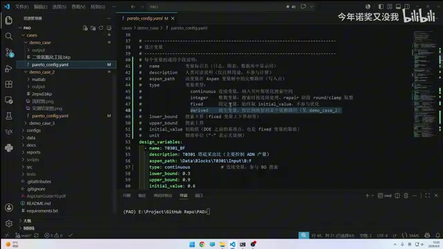
Each design variable requires: name, description, Aspen node path, variable type (integer int or continuous float), upper/lower bounds, and initial value.

Using the acetonitrile distillation section case as an example:

• Tray theoretical stage ratio (BF value): Continuous, range 0.03–0.09, initial value 0.06
• Reflux ratio: Continuous, also requiring a defined search range

If a variable should not participate in optimization, it can be set as fixed (fixed), and the system will skip it during the optimization process.

Objective Function Setup

Objective functions have a similar structure to design variables, requiring node paths and optimization directions. For example:

• ADN production: Maximize
• Reboiler heat duty: Minimize

When multiple objectives exist, the system automatically switches to multi-objective optimization mode and begins Pareto front search. The Pareto Front is a core concept in multi-objective optimization, referring to the set of all non-dominated solutions in the objective space. A solution is called non-dominated when no other solution exists that is superior in all objectives simultaneously. In chemical optimization, maximizing production and minimizing energy consumption are often conflicting goals—the Pareto front provides engineers with a set of optimal trade-off solutions from which decision-makers can choose based on actual needs. Common multi-objective optimization algorithms include NSGA-II and MOEA/D, while this project's multi-objective Bayesian optimization efficiently approximates the Pareto front through extended acquisition functions (such as EHVI, Expected Hypervolume Improvement).

Constraint Configuration

Constraints are defined through comparison operators (≥, ≤, =, etc.) and thresholds. For example, requiring product purity ≥ 0.99—if the simulation converges but doesn't satisfy the constraint, that operating condition is marked as an "infeasible point."

Node Database: First-Run Cost and Reuse Mechanism

One particularly elegant design in the project is the node path caching mechanism. Each piece of equipment in Aspen contains numerous parameter nodes, and the first run requires the system to traverse and search all relevant node paths—a process that is often very time-consuming.

However, search results are stored in a .db file. On subsequent runs, the system reads paths directly from the database, dramatically improving speed. This is similar to memoization in computing—results computed once are directly reused, avoiding redundant work. From a computer science perspective, memoization is one of the core techniques of dynamic programming, avoiding repeated calculations by caching previously computed results. In this project, Aspen's node tree structure resembles a file system's directory tree, where each piece of equipment (such as distillation columns or heat exchangers) contains hundreds or even thousands of parameter nodes. The time complexity of the first traversal of this tree is proportional to the total number of nodes, but after persisting results to a lightweight database, subsequent query time complexity drops to O(1) or O(log n)—achieving orders-of-magnitude performance improvement.

The "depth" parameter in the configuration controls the level of node search: greater depth means more comprehensive searching but slower first runs. A setting of 2–4 is generally recommended, with 4 being a very deep search level.

Bayesian Optimization and Surrogate Model Principles

Intuitive Understanding of Surrogate Models

Imagine standing in a pitch-dark room with an undulating continuous surface in front of you, and you need to find the highest point. You have a limited number of glow balls—each one thrown reveals the height at that position, but each throw has a cost.

Your goal is to use the fewest glow balls possible to accurately map the surface and find the highest point. This is exactly the core idea behind Bayesian optimization:

1. DOE Phase (Initial Sampling): First throw out a batch of glow balls to establish initial understanding of the solution space. DOE (Design of Experiments) is a statistical methodology for systematically planning experiments. In the optimization context, the DOE phase aims to uniformly distribute initial sampling points across the search space, providing sufficient training data for the surrogate model. Common sampling strategies include Latin Hypercube Sampling, Sobol sequences, and orthogonal designs. Good initial sampling prevents the surrogate model from developing severe bias early on, thereby accelerating subsequent optimization convergence.

2. Iterative Optimization Phase: Based on existing information, intelligently select the next sampling point, balancing between "exploring unknown regions" (Exploration) and "exploiting known high points" (Exploitation). This Exploration-Exploitation Trade-off is the key characteristic distinguishing Bayesian optimization from traditional optimization methods—the acquisition function automatically achieves this balance by quantifying the potential value of each candidate point.

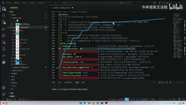
Early Stopping Mechanism and Patience Value Settings

The early stopping strategy in the configuration originates from a gating system in a top-conference paper. When several consecutive generations show no improvement, the system automatically stops optimization to avoid wasting computational resources. Early Stopping was originally widely used in deep learning training to prevent overfitting. In the optimization domain, early stopping strategies monitor the improvement trend of the objective function to determine whether to continue iterating. The introduction of a Gating System makes the stopping decision more intelligent—it considers not only the number of consecutive generations without improvement but may also incorporate improvement magnitude, search space coverage, and other multi-dimensional information for decision-making. This mechanism has significant practical value in industrial scenarios with limited computational resources.

However, it's important to note that early stopping may miss breakthrough improvements in later stages. Users need to adjust the "patience" value based on practical experience—that is, how many generations without improvement to tolerate before triggering a stop.

Information Utilization from Infeasible Points

Based on methods from the literature, the system labels converged points as positive samples and non-converged points as negative samples. Negative samples also carry valuable information—they tell the optimizer to "stay away from these regions." This is similar to the positive and negative poles of a magnet, forming attraction and repulsion fields that jointly guide the search direction toward the feasible region.

From a theoretical perspective, in constrained optimization, traditional methods often simply discard sampling points that don't satisfy constraints. However, classification-based constraint handling methods (such as Probability of Feasibility) model feasibility as an independent classification problem, using all sampling points (including infeasible ones) to learn the boundary of the feasible region. This approach trains an additional Gaussian Process classifier to estimate the feasibility probability of any point, multiplying it with the expected improvement as the final acquisition function value—naturally guiding the search toward regions that are both feasible and promising. This means that even failed simulations are not wasted; every computation provides valuable information to the optimizer.

Practical Demonstration: From Single-Objective to Multi-Objective Optimization

Single-Objective Optimization Case

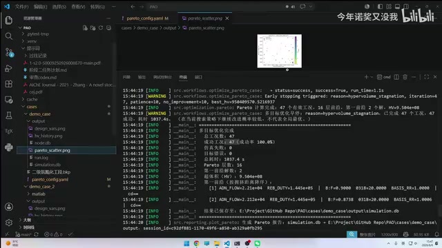
Using the acetonitrile distillation section as an example, simultaneously optimizing ADN production and reboiler heat duty. The first run's node scanning is slower, but subsequent iterations take only a few seconds each. The entire optimization process converges after approximately 30 iterations.

Results include three key outputs:

• Pareto front plot: Visually displays trade-off relationships between multiple objectives. Each point in the plot represents a non-dominated solution, allowing engineers to select the most appropriate operating point between production and energy consumption based on actual production needs.
• Convergence curve: Convergence can be observed starting around generation 20, indicating that the surrogate model has adequately fitted the global trend of the objective function.
• Variable distribution plot: Shows the parameter regions favored by optimal solutions, helping users determine whether search ranges need adjustment. If optimal solutions cluster near boundaries, it typically means the search range is too narrow and boundaries need to be expanded.

Complex Multi-Objective Optimization Case

The second case involves three-product separation of n-propanol, isobutanol, and water, containing three distillation columns, 14 design variables, and multiple constraints—significantly higher complexity. Fourteen design variables mean the search space is 14-dimensional, which is virtually impossible to handle with traditional exhaustive search—even if each variable takes only 10 discrete values, the number of combinations reaches 10^14. The sample efficiency advantage of Bayesian optimization is particularly evident in such high-dimensional scenarios.

Thanks to existing node caching, the second run only needs to search 3 nodes before starting. The system also includes a feasibility pre-check function: if no converging point is found after 30 consecutive attempts, the current search space configuration is deemed invalid, prompting users to adjust parameter ranges. This design prevents users from waiting extended periods for invalid results under incorrect configurations. Ultimately, this case found the optimal solution in 71 iterations, approximately 7 minutes.

Future Outlook: AI Agents Empowering Chemical Process Design

The project will subsequently introduce an Engine module (AI Agent), planned to achieve the following capabilities:

• Automatically reading chemical literature and extracting process parameters
• Intelligent tuning and parameter recommendations
• Automatically building Aspen process frameworks
• Superstructure optimization (addressing the current temporary TC calculation approach)

Superstructure Optimization is a classic problem in chemical process synthesis, referring to the use of mathematical programming methods to select the optimal process topology from a superstructure containing all possible process routes. This involves not only operating parameter optimization but also equipment selection, connection methods, and process architecture decisions—a higher-level design problem than parameter optimization.

This will upgrade the project from "manual configuration + automated optimization" to "fully autonomous AI-driven process development," truly achieving an intelligent closed loop for chemical process design. By combining the literature comprehension capabilities of large language models with the efficient search capabilities of Bayesian optimization, future chemical process design is expected to transition from the traditional "experience-driven" paradigm to a new "data and AI-driven" paradigm.

Key Takeaways