Neural Networks from Scratch: A Deep Dive into the Fundamentals from Linear Regression to Gradient Descent

A ground-up derivation of neural network fundamentals from linear regression to backpropagation.
This article builds neural network understanding from the ground up, starting with linear regression and progressing through logistic regression, gradient descent, and feature combination. It covers Sigmoid functions, cross-entropy loss, activation function theory via Taylor expansion, and the chain rule behind backpropagation, connecting each concept to modern LLM architectures.
Introduction: Why Bother Understanding Neural Networks at the Lowest Level?
Mastering the underlying principles of deep learning is the essential path from being an LLM application developer to becoming an LLM solution architect. Only by truly understanding model architecture and training principles can you design high-performance, cost-effective solutions and confidently tackle the scaling challenges of trillion-parameter models.
This article starts from the most basic linear regression and progressively derives logistic regression, gradient descent, and ultimately the core mechanisms of neural networks — feature combination and backpropagation. These topics are not only must-know material for big tech interviews but also the foundation for understanding modern LLM architectures like Transformer and Attention.
Linear Models: From Linear Regression to Logistic Regression
Linear Regression: The Simplest Prediction Model
The core idea of linear regression is highly intuitive: the predicted value Y has a linear relationship with the input features, meaning each feature X's change has a proportional impact on Y. The mathematical expression is:
$$Z = W_1X_1 + W_2X_2 + ... + W_nX_n + b$$
Here, W represents the weight parameters and b is the bias term — together they determine the model's predictive capability.
The history of linear regression dates back to the early 19th century, when Gauss and Legendre independently proposed the method of least squares. It is not only the starting point of machine learning but also a cornerstone of statistics as a whole. In the deep learning era, the idea of linear regression remains ubiquitous — the linear projection layers in Transformers (used to generate Q, K, V matrices) are essentially parallel computations of multiple linear regressions. Understanding the physical meaning of weight W in linear regression — i.e., each feature's contribution to the prediction — helps in later understanding the semantic role of weight matrices in Attention.
Logistic Regression: Add a Sigmoid and You Get a Classifier
The only difference between linear regression and logistic regression is a Sigmoid function. By wrapping the linear regression output Z with a Sigmoid:
$$\hat{Y} = \sigma(Z) = \frac{1}{1 + e^{-Z}}$$
The Sigmoid function maps any real number to the open interval (0, 1), and the output can be interpreted as a probability. When the predicted probability is greater than 0.5, it's classified as positive; when less than 0.5, it's classified as negative — though this 0.5 threshold is subjectively set and can be adjusted based on business requirements.
It's worth noting that while the Sigmoid function held a central position in the history of neural networks, it has been gradually replaced by ReLU (Rectified Linear Unit) and its variants in modern deep networks. The reason is that Sigmoid suffers from the vanishing gradient problem: when the absolute value of the input is large, the derivative of Sigmoid approaches 0, causing gradients to decay layer by layer during backpropagation, making it nearly impossible to update parameters close to the input layer. The ReLU function $f(x)=\max(0,x)$ has a constant derivative of 1 in the positive region, effectively mitigating this issue. However, in the LLM domain, more sophisticated activation functions like GELU (Gaussian Error Linear Unit) and SwiGLU are becoming mainstream choices — for example, the LLaMA model family uses the SwiGLU activation function.
Gradient Descent: The Core Engine of Model Learning
Loss Functions and Parameter Updates
Model parameters W are randomly initialized at the start, and we need a method to progressively optimize them. For linear regression, the loss function uses mean squared error:
$$L = (\hat{Y} - Y)^2$$
We want this loss to keep decreasing, and the only way to change the loss is to adjust W. How exactly? By computing the partial derivative with respect to W:
$$\frac{\partial L}{\partial W_1} = 2(\hat{Y} - Y) \cdot X_1$$
Then update the parameters in the opposite direction of the gradient:
$$W_1 = W_1 - \mu \cdot \frac{\partial L}{\partial W_1}$$
Here μ is the learning rate. If the learning rate is too small, convergence is slow and time-costly; if too large, parameters oscillate back and forth and fail to converge to the optimal solution.
What's described above is the most basic Batch Gradient Descent. In practice, there are several important variants. Stochastic Gradient Descent (SGD) computes the gradient using only one sample at a time — fast but noisy. Mini-batch SGD strikes a balance and is the most commonly used approach today. Going further, the Adam optimizer combines momentum and adaptive learning rate, automatically adjusting the learning rate for different parameters, and has become the standard for LLM training. When training models with hundreds of billions of parameters like GPT-3, additional strategies such as learning rate warmup, cosine annealing, mixed-precision training, and gradient accumulation are required to achieve stable convergence across thousands of GPUs.
The Loss Function for Logistic Regression: Cross-Entropy
The loss function for logistic regression is no longer mean squared error but Cross-Entropy:
$$L = -[Y \cdot \log\hat{Y} + (1-Y) \cdot \log(1-\hat{Y})]$$
Cross-entropy essentially measures the difference between two probability distributions. Since logistic regression predicts probabilities, using cross-entropy to measure the distance between predicted probabilities and true labels is mathematically more appropriate.
Cross-entropy originates from information theory, founded by Claude Shannon in 1948. In information theory, entropy measures the uncertainty of a probability distribution, while cross-entropy measures the average number of bits needed to encode one distribution using another. When the predicted distribution perfectly matches the true distribution, cross-entropy equals the entropy of the true distribution, reaching its minimum. Compared to mean squared error, the advantage of cross-entropy in classification tasks is that when predictions deviate severely from true labels, cross-entropy produces larger gradients, driving the model to correct errors faster. This property is especially important in LLM pretraining — the pretraining objective of the GPT series is to minimize the cross-entropy loss for next-token prediction.
The most critical advantage of gradient descent is its universality — this method pervades the entire AI field, from traditional machine learning to today's LLMs and multimodal models. It's not limited to any specific model form; as long as you can differentiate the loss function, you can use it for optimization.
From Logistic Regression to Neural Networks: The Art of Feature Combination
The Linear Inseparability Problem
Logistic regression essentially draws a line (or hyperplane) to separate data. But when data is linearly inseparable — no matter how you draw the line, you can't completely separate the two classes — logistic regression is helpless.
A naive solution is to manually construct new features. For example, if the original features are X1 and X2, we define X3 = X1 × X2, lifting the problem from 2D to 3D, where a plane might be able to separate the two classes.
Good Features Matter More Than Good Models
Effective classification relies on three things: highly discriminative features, a large number of features, and rich feature combinations. It's like a bad hand of cards that can still win if it forms a straight. But in practice, the first two are often fixed — you get whatever features the data provides. The real room for improvement lies in the third: various combinations of features.
However, when the number of features reaches hundreds, manual combination becomes virtually impossible. This gave rise to neural networks — a method for automatic feature combination.
The ability of neural networks to automatically combine features marks a major paradigm shift in machine learning, from the "feature engineering" era to the "representation learning" era. In traditional machine learning, data scientists spent enormous amounts of time manually designing features (e.g., TF-IDF and bag-of-words models in NLP), and model performance was highly dependent on the quality of feature engineering. The core breakthrough of deep learning is letting the model learn the optimal representation of data on its own. This idea has been taken to the extreme in LLMs — BERT learns universal language representations through pretraining, GPT learns generative text representations through autoregressive pretraining, and CLIP learns multimodal representations that align images and text. In essence, modern LLMs are ultra-large-scale automatic feature combiners.
Neural Networks: Automated Feature Combination
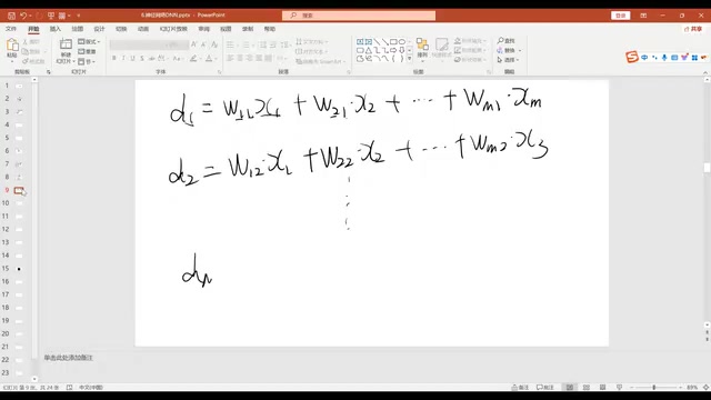
The core idea of neural networks is to let m original features generate new combined features through weighted summation. Each new feature is a linear combination of the original features:
$$d_1 = W_{11}X_1 + W_{21}X_2 + ... + W_{m1}X_m$$ $$d_2 = W_{12}X_1 + W_{22}X_2 + ... + W_{m2}X_m$$
Different weight combinations produce different feature representations. In matrix form, this can be written concisely as: D = W · X, where W is an M×m parameter matrix. Matrix operations essentially compress a large number of weighted summations into a single concise formula.
Activation Functions: Why Are Nonlinear Transformations Indispensable?
Understanding Nonlinear Activation Through Taylor Expansion
Linear combination alone is not enough — a nonlinear transformation (activation function), such as Sigmoid, must be applied to the combination result. Why?
According to the Taylor formula, any function can be expanded as a weighted sum of polynomials. If the activation function f is Sigmoid, all orders of its derivatives are non-zero. When we perform a Taylor expansion of $f(W_{11}X_1 + W_{21}X_2 + W_{31}X_3)$, the second-order terms will inevitably include cross terms like $X_1 \cdot X_2$, $X_1 \cdot X_3$, $X_2 \cdot X_3$, and even higher-order combination terms.
This means that nonlinear activation functions inherently possess the mathematical capability for higher-order feature combination, without any manual design. This is the mathematical foundation of neural networks' powerful expressive capability.
From a broader theoretical perspective, this is closely related to the Universal Approximation Theorem. The theorem states that a single-hidden-layer feedforward neural network with sufficiently many hidden neurons, using a nonlinear activation function, can approximate any continuous function to arbitrary precision. In other words, without nonlinear activation functions, no matter how many layers the network has, its expressive power is equivalent to a single-layer linear model — because the composition of multiple linear transformations is still a linear transformation. Nonlinear activation functions are the key to breaking this limitation.
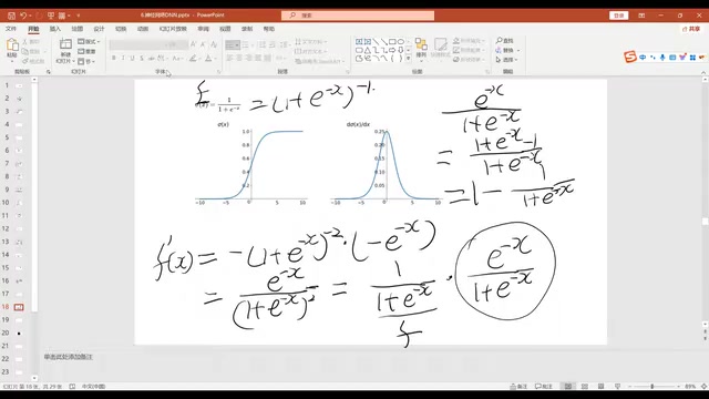
Deriving the Sigmoid Derivative
The derivative of the Sigmoid function is a high-frequency interview question. The derivation is as follows:
$$f(x) = \frac{1}{1 + e^{-x}}$$
$$f'(x) = \frac{e^{-x}}{(1 + e^{-x})^2} = f(x) \cdot (1 - f(x))$$
This result is remarkably elegant: the derivative of Sigmoid can be expressed in terms of the function value itself. This is extremely convenient for backpropagation computations, and all subsequent derivations involving Sigmoid will directly use this result.
Complete Neural Network Structure and Backpropagation Derivation
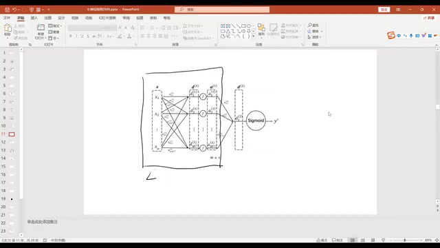
Building a Two-Layer Neural Network
Take the simplest two-layer neural network as an example: the input layer has two features X1 and X2, the hidden layer has 3 neurons (A1, A2, A3), and the output layer performs binary classification.
The computation process for each hidden layer neuron is:
- Weighted summation: $Z = W_1X_1 + W_2X_2 + b$
- Activation transformation: $A = \sigma(Z)$
The hidden layer outputs A1, A2, A3 serve as new features, which are then fed into the output layer for logistic regression to produce the final prediction $\hat{Y}$.
The first half is feature combination, and the second half is a standard logistic regression. All weight parameters are learned through gradient descent — we only need to tell the network "you need to combine features," and the training task and data determine how to combine them and what values the weights should take.
The Chain Rule: The Mathematical Foundation of Backpropagation
The key to solving neural network parameters lies in the chain rule. For composite functions $z = g(k \cdot y)$, $y = f(w \cdot x)$:
$$\frac{\partial z}{\partial w} = \frac{\partial z}{\partial y} \cdot \frac{\partial y}{\partial w}$$
This is the mathematical essence of the backpropagation algorithm: starting from the output layer, gradients are propagated layer by layer along the computational graph, where each layer's gradient is the product of the subsequent layer's gradient and the current layer's local gradient.
The backpropagation algorithm was formally proposed and popularized by Rumelhart, Hinton, and Williams in their seminal 1986 paper, and is considered one of the most important algorithmic breakthroughs in the history of deep learning. Its core idea is to use the chain rule to compute gradients layer by layer from the output to the input, avoiding redundant calculations. Modern deep learning frameworks (such as PyTorch and TensorFlow) automatically implement backpropagation through computational graphs: during forward propagation, the computational graph is constructed and every operation is recorded; during backpropagation, the graph is traversed in reverse to automatically compute gradients for all parameters. This is what happens behind the scenes when you call loss.backward() in PyTorch. Understanding the manual derivation of backpropagation helps you quickly identify the root cause of gradient anomalies (such as gradient explosion or vanishing gradients) during model debugging.
Once you've mastered the chain rule and the Sigmoid derivative, you have the ability to manually derive gradients for any neural network. Nowadays, big tech interviews may even require you to derive gradients for the Transformer's Attention mechanism — if you can't even derive the basic Sigmoid gradient, more complex structures are out of the question.
Summary
From linear regression to logistic regression to neural networks, the evolution follows a clear trajectory: linear model → add Sigmoid to create a classifier → add hidden layers for feature combination → add nonlinear activation for higher-order expressive power → use gradient descent for end-to-end learning of all parameters.
These fundamentals may seem simple, but they are the underlying principles for understanding DNN, Attention, Transformer, and the entire LLM ecosystem. Mastering these basics will give you confidence whether you're facing technical interviews or designing real-world system architectures.
Key Takeaways
Related articles
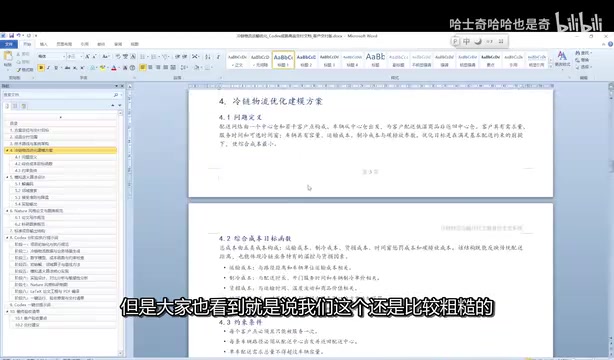
Building a Cold Chain Logistics Optimization Research Project with Codex: A Complete Workflow from Scratch to PDF Paper
Learn how to use OpenAI Codex to build a complete cold chain logistics optimization research project from scratch, including simulated annealing implementation, experiments, figures, and LaTeX paper compilation.
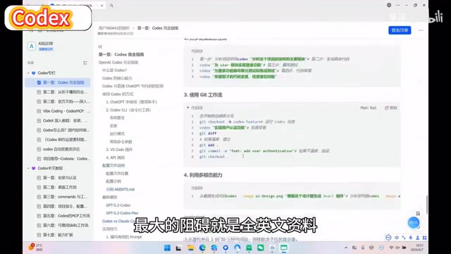
Codex Beginner's Practical Guide: Master Core AI Programming Skills in One Weekend
OpenAI Codex beginner's practical guide covering environment setup, code generation, bug fixing, and project refactoring. Includes efficient learning tips and Prompt techniques for fast AI programming mastery.

AI Agent Systematic Learning Path: From Zero to Independent Development
A systematic AI Agent learning path covering core principles, Prompt engineering, RAG, multi-Agent collaboration, and hands-on projects for beginners.