AI Data Center Load Forecasting: How Probabilistic Calibration and Temporal Structure Affect Grid Decisions

448-GPU measured data shows AI load forecasting must jointly address calibration, temporal structure, and decisions to avoid high reserve costs.
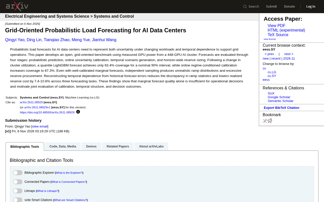
Based on measured power data from a 448-GPU AI cluster, this study builds an open benchmark for grid operations covering probabilistic forecasting, online calibration, temporal scenario generation, and reserve planning. After utilization shifts, quantile LightGBM's nominal 90% interval covers only 63.4%, while online regime-conditioned calibration raises coverage to 87.3%. Independent sampling from marginals distorts ramp rates and causes excess reserves; reconstructing temporal dependence cuts actual reserve costs by 7.4%-10.6% across three tasks. The core conclusion: marginal forecast quality alone cannot support operational decisions—calibration, temporal structure, and decision outcomes must be evaluated jointly.
Why AI Data Center Load Forecasting Requires Dedicated Research
The power fluctuations of AI training clusters are fundamentally different from those of traditional data centers. GPU-intensive workloads produce sharp power swings during task scheduling, checkpoint writes, communication synchronization, and similar phases, and these swings vary dynamically with model size, parallelism strategy, and cluster utilization. Grid operators need to anticipate these loads hours or even days in advance in order to arrange reserve capacity and frequency regulation resources.
However, a study based on measured data from an AI cluster with 448 GPUs points out that traditional probabilistic forecasting methods alone are far from sufficient. The paper builds an open benchmark oriented toward grid operations, using measured GPU power data across four stages: probabilistic forecasting, online uncertainty calibration, temporal scenario generation, and full-horizon reserve capacity planning. Its core conclusion is that marginal forecasting quality alone is insufficient to support operational decisions; calibration, temporal structure, and decision outcomes must be evaluated jointly.
Probabilistic Calibration: Fixing Coverage from 63.4% to 87.3%
Why Does a Nominal 90% Interval Cover Only 63.4%?
After cluster utilization changed, the research team used a quantile LightGBM model for probabilistic forecasting. The nominal 90% prediction interval actually covered only 63.4% of observations — meaning that when the grid reserves capacity based on this interval, it will face insufficient capacity risk during a large number of periods.
The root cause of this inaccuracy is distribution shift: when the AI cluster switches from one utilization state to another, the quantile relationships in the historical training data no longer hold. The model does not "realize" that it has entered a new operating regime.
Quantile regression and quantile LightGBM: Quantile regression does not predict the conditional mean, but directly estimates the conditional value of the target variable at a given quantile (e.g., 5%, 50%, 95%). Quantile LightGBM changes the loss function of gradient boosted trees to pinball loss (quantile loss), enabling the model to output predictions at multiple quantiles and thereby construct prediction intervals. A nominal 90% interval is typically formed by the 5% and 95% quantiles. However, quantile regression assumes that training data and test data are identically distributed; when the operating conditions of an AI cluster drift, the quantile mapping learned from history becomes invalid, causing interval coverage to fall far below the nominal level. This is precisely the technical root cause of the 63.4% coverage in the article.
The Remedial Effect of Online Regime-Conditioned Calibration
The paper adopts online regime-conditioned calibration to dynamically correct the quantiles. After calibration, the actual coverage of the same nominal 90% interval rises to 87.3%, close to the nominal level. This result shows that AI load forecasting systems must have online adaptive capability; the approach of training once statically and deploying will quickly fail when cluster conditions change.
It is worth noting that 87.3% is still below 90%, indicating that calibration is not perfect, but it has substantially narrowed the deviation. For reserve capacity planning, this degree of correction is sufficient to significantly change decision quality.
Online regime-conditioned calibration: Its core idea is to dynamically adjust quantile outputs after forecasting and before decision-making, based on the deviation between recently observed actual values and predicted values. Specific approaches typically include: identifying the current operating regime (e.g., cluster utilization range), and within that regime using the residual distribution from a recent window to remap quantiles so that calibrated interval coverage approaches the nominal value. Unlike static training, this method continuously updates calibration parameters and can track distribution shift. The increase in coverage from 63.4% to 87.3% in the article is precisely because regime-conditioned calibration reduced the deviation caused by distribution shift, but did not completely eliminate it, indicating that calibration window length and regime partition granularity still affect performance.
Temporal Structure: Why Independent Sampling Leads to Excess Reserve Procurement
Correct Marginal Distribution Does Not Mean Reasonable Scenarios
Even when marginal forecasts are well calibrated, the research found a second pitfall: if temporal scenarios are generated by independent sampling from the calibrated marginal distribution, the resulting ramp-rate distribution becomes severely distorted. Independent sampling assumes that forecast errors at adjacent time steps are uncorrelated, but errors in real loads exhibit clear temporal dependence — deviations over consecutive time steps often accumulate in the same direction.
This distortion propagates directly to the decision side: the grid calculates reserve requirements based on an unrealistic ramp distribution, resulting in excessive procurement of reserve capacity and higher operating costs.
Marginal distribution and joint distribution: The marginal distribution describes the probability distribution of forecast error at a single time point, whereas temporal scenario generation requires the joint distribution of errors across multiple time points. Independent sampling assumes that errors at different times are mutually independent, i.e., the joint distribution equals the product of the marginals. But real load forecast errors typically exhibit autocorrelation: errors over consecutive time steps often accumulate in the same direction, forming ramp events. Independent sampling destroys this correlation, causing the magnitude and frequency of ramps in generated scenarios to be underestimated or overestimated. The article points out that the ramp-rate distribution is severely distorted precisely because independent sampling erases the temporal dependence structure of errors, thereby causing scenario-based reserve requirement calculations to deviate from reality.
Reconstructing Temporal Dependence from Historical Forecast Errors
The paper's solution is to reconstruct the temporal dependence structure from historical forecast errors and then use it for scenario generation. After reconstruction, the deviation in ramp statistics is significantly reduced, and across three forecasting tasks, actual reserve costs fall by 7.4% to 10.6%.
The insight from this result is that evaluation metrics for probabilistic forecasting (such as coverage and pinball loss) only measure marginal quality, whereas operational decisions care about joint behavior along temporal paths. There is a systematic gap between the two that requires dedicated methods to bridge.
Temporal scenario generation and ramp rate: Temporal scenario generation refers to producing multiple future load paths that conform to historical statistical characteristics, for use in stochastic optimization or reserve capacity planning. Common methods include covariance matrix methods, Copula models, and bootstrap residual resampling. Reconstructing temporal dependence from historical forecast errors in the article essentially means estimating the autocorrelation structure of the error series (e.g., via an AR model or empirical Copula) and then preserving that structure when generating scenarios. Ramp rate refers to the difference in load between adjacent time steps, and its distribution directly affects reserve requirements: the more severe the ramp, the more flexible resources the system needs. After reconstructing temporal dependence, the ramp statistics in scenarios are closer to measured values, thereby avoiding excess reserve procurement caused by independent sampling.
Practical Implications for Grid Operations and AI Infrastructure
For grid operators, AI data centers are not ordinary large-load customers. Their power trajectories are strongly driven by training task scheduling and exhibit regime-switching non-stationary characteristics. If traditional load forecasting processes are retrained only quarterly or annually, it is difficult to keep up with this pace of change; online calibration must be incorporated into standard workflows.
For AI cluster operators, providing the grid with more accurate load predictability may become a condition for participating in demand response or obtaining better electricity pricing. The 448-GPU cluster data used in the paper shows that measured power data is sufficient to support the construction of such forecasting benchmarks; there is no need to wait for hyperscale clusters to act.
For forecasting method research, the benchmark's four evaluation stages provide a reusable framework: first look at probabilistic forecasting, then online calibration, then temporal scenarios, and finally reserve decisions. If any link is missing, forecasting metrics that look good may fail in actual operations.
The paper's final point deserves repetition: marginal forecasting quality alone is insufficient to support operational decisions; calibration, temporal structure, and decision outcomes need to be evaluated jointly. For AI computing infrastructure that is rapidly expanding, this conclusion has strong real-world relevance.
One-line Summary
Measured data from 448 GPUs shows that AI load forecasting must jointly address calibration, temporal structure, and decisions; otherwise reserve costs remain high.
Paragraph Summary
Based on measured power data from an AI cluster with 448 GPUs, this article builds an open benchmark oriented toward grid operations, covering four stages: probabilistic forecasting, online calibration, temporal scenario generation, and reserve capacity planning. The study finds that after cluster utilization changes, the actual coverage of a nominal 90% interval from quantile LightGBM is only 63.4%, and online regime-conditioned calibration can raise it to 87.3%. Even when marginal forecasts are well calibrated, generating temporal scenarios by independent sampling from the marginal distribution still distorts the ramp-rate distribution, leading to excess reserve procurement; after reconstructing temporal dependence from historical forecast errors, actual reserve costs across three forecasting tasks fall by 7.4% to 10.6%. The core conclusion is that marginal forecasting quality alone is insufficient to support operational decisions; calibration, temporal structure, and decision outcomes must be evaluated jointly.
Related articles

Claude Code in Practice: Installation, MCP, Skills, and SubAgent Techniques
From npm installation and CC Switch login bypass to permission modes, MCP, Skills, SubAgent, and CLAUDE.md configuration—a systematic guide to practical Claude Code techniques.

FastAPI Learning Path: From Beginner to AI Project Practice
A Bilibili creator recommends *FastAPI Web Development: From Beginner to Advanced with Practical Projects*. This article outlines the FastAPI learning path: target audience, the 15-chapter six-part structure, project-driven learning, and practical directions from web backend to AI Agents, helping beginners avoid detours.

Reverse-Engineering Taobao's sign Signature Parameter with AI in 10 Minutes: A Practical Walkthrough
Based on a Bilibili hands-on demo, this article explains how to combine DeepSeek with vision models to automatically reverse-engineer Taobao's sign signature parameter, track dynamic titter and token values, and successfully scrape product data within ten minutes—while analyzing the capability boundaries and compliance risks of AI Agents in crawler reverse engineering.