GRPO Reinforcement Learning Explained: Group Relative Policy Optimization That Teaches LLMs to Reason

GRPO replaces the value network with in-group relative comparison for the same question, efficiently optimizing reasoning via standardized advantages and clipping.
Based on StatQuest's minimalist explanation, this article systematically covers GRPO's principles and engineering details. GRPO's core is constructing advantages by comparing a group of responses to the same prompt, avoiding a value network of the same scale as the policy and greatly reducing memory and engineering complexity. The process: high-temperature sampling of a group, arbitrary scoring, in-group standardization for advantages, then plugging into the loss for backpropagation. The author breaks down the loss: clipping limits advantage scaling to [1-ε,1+ε], amplifying positive advantages and pulling negative ones toward zero; the first iteration has ratio 1 and loss 0, with scaling only effective from the second round; the KL term constrains new-vs-old distribution distance and its weight can be lowered or zeroed. Finally, reward scale doesn't matter, but in-group discrimination and sampling temperature must be coordinated—otherwise advantages approach zero and gradients fail.
GRPO (Group Relative Policy Optimization) is a reinforcement learning algorithm that has drawn considerable attention in recent years for training the reasoning capabilities of large models. It sidesteps the hassle of training a separate value network (critic) required by traditional PPO methods, instead constructing advantage signals by comparing a group of responses to the same prompt against one another. Josh Starmer of StatQuest breaks GRPO down quite clearly with a minimalist mathematical example. Below, building on his explanation, we walk through the core logic and engineering details of this method in full.
Why GRPO Is Needed: Starting from In-Group Comparison
The core motivation behind GRPO can be summed up in one sentence: rather than training an additional value model to estimate "how good this answer is," just have the model generate a group of answers to the same question and compare them against each other within the group. Under this design, the advantage function no longer depends on an absolute baseline but is computed relative to the other responses in the same group—this is precisely what the "G" (Group) and "R" (Relative) stand for.
The specific process has four steps: for each training prompt, generate a group of responses using a relatively high temperature; score each response using any scoring mechanism (a calculator or a stronger model); standardize the rewards within the group to obtain advantage values; and plug the advantage values into the GRPO loss function to perform policy optimization via backpropagation.
The temperature setting is a prerequisite for this process. When temperature is set to 1, the model's output diversity is noticeably higher than under low-temperature settings—this is exactly why GRPO needs a group of diverse responses (some correct, some wrong). The higher the temperature, the greater the chance of sampling low-probability tokens, and the more sufficient the diversity of samples within the group.
Temperature is a sampling parameter used during large model generation. It acts on the logits output by the model: they are first divided by the temperature coefficient T, then passed through softmax to obtain a probability distribution. At T=1, the model's original distribution is preserved; T<1 sharpens the distribution, making high-probability tokens more likely to be selected and outputs more deterministic and conservative; T>1 flattens the distribution, giving low-probability tokens a greater chance of being sampled and making outputs more random and diverse. GRPO needs a group of responses with both correct and incorrect answers to form an effective comparison, so temperature is typically raised (e.g., 0.8–1.2) to ensure sufficient diversity within the group. Too low a temperature causes responses within the group to be highly similar, advantages to approach zero, and gradient signals to vanish.
Why the Reward Value Itself Doesn't Matter: Standardization and Advantage
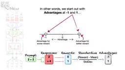
Josh Starmer uses a toy language model with only four tokens (2, +, =, 4) to demonstrate the entire process. The scoring rule is 1 for a correct answer and 0 for an incorrect one, but the video specifically emphasizes that the concrete numerical value of the reward has almost no effect on the result, because standardization is performed immediately afterward.
$$\hat{A}_i = \frac{r_i - \text{mean}(r)}{\text{std}(r)}$$
After standardization, the better response within the group receives a positive advantage and the worse response a negative advantage, centered on zero. The video demonstrates with several sets of different reward values: when rewards are 0 and 1, when they are -2 and -1, and when they are -0.5 and 1.5, the standardized advantages are all -1 and 1. In other words, as long as the good answer's reward is higher than the bad answer's, standardization automatically separates the good from the bad, and there is no need to agonize over how to set the reward scale in engineering practice.
This design is very valuable for practical training. Reward signals may come from rule-based verification, code sandbox execution results, or another model's scoring, with vastly different scales, but after in-group standardization they can all enter the same optimization framework.
Breaking Down the GRPO Loss Function Term by Term
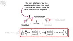
The full formula looks complex, but we can first grasp the main structure. The video decomposes the loss function into three layers: the first layer is the clipping function, which limits the scaling factor of the advantage to the interval $[1-\epsilon, 1+\epsilon]$, where $\epsilon$ is typically 0.1 or 0.2; the second layer is the importance sampling ratio, i.e., the ratio of the current policy's probability to the old policy's probability for the same token; the third layer averages over tokens and over responses within the group, and finally takes the negative sign to obtain the loss.
The intuitive meaning of clipping is: relax the room for amplifying positive advantages while constraining the scaling magnitude of negative advantages. In other words, the model is encouraged to further reinforce good answers, but the penalty on bad answers has an upper bound, preventing a single update from pulling the probability distribution too far.
The "Idling" Phenomenon in the First Iteration
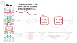
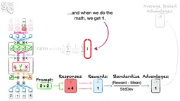
One easily confusing detail: right after initialization, before any parameters have been updated, the current policy is entirely identical to the old policy, and the ratio is 1 everywhere. Since 1 falls within $[1-\epsilon, 1+\epsilon]$, the clipping function returns 1 as-is, and the advantage is not scaled. The result computed in the video is: the advantages of the two responses are -1 and 1 respectively, which average to 0, and the loss is also 0.
This is not a contradiction. A loss of 0 is merely the value at the current parameter point; by taking the derivative with respect to the parameters and moving along the gradient descent direction, the loss can continue to decrease to negative values. GRPO's scaling effect only truly manifests in the second round—at which point the ratio begins to deviate from 1.
The Second Round: The Ratio Begins to Deviate from 1
After the parameter update, the model's probability for the incorrect answer "2" drops from 0.24 to 0.20, making the ratio 0.83; the probability of "=" in the correct answer rises from 0.22 to 0.45, making the ratio 2.05, which exceeds the upper bound and is clipped to 1.2. The video also handles the multi-token case: the second response contains two tokens, "=" and "4", which come from different conditional probability distributions and require computing the ratio separately for each and then averaging.
The result is: the advantage of the bad answer is pulled from -1 toward -0.83, the advantage of the good answer is amplified to 1.17, and the loss after averaging is -0.17. The loss drops from 0 to -0.17, indicating that optimization is progressing. This numerical trajectory precisely corresponds to GRPO's training dynamics of "suppressing incorrect paths and reinforcing correct paths."
The importance sampling ratio is a core component of the PPO family of algorithms, defined as the ratio of the current policy's probability to the behavior policy's (i.e., the old policy at the time the data was sampled) probability for the same action: $\rho = \pi_\theta(a|s) / \pi_{\theta_{old}}(a|s)$. It is used to correct for the distribution shift introduced by "data collected by the old policy but optimized with the new policy," making off-policy updates unbiased in expectation. A ratio greater than 1 indicates the new policy favors that token more, and less than 1 the opposite. GRPO follows this mechanism but drops the granularity of actions to the token level, computing token by token for multi-token responses and then averaging.
The KL Divergence Term: Don't Let the Model Drift Too Far
The formula also contains an often-overlooked KL divergence term, used to measure the distance between the entire original probability distribution and the new distribution, not just the probability difference of a single token. In theory, GRPO should only make subtle adjustments and should not drastically rewrite the original language capabilities—the KL term is the "reins" that impose this constraint. The video mentions that in practice the weight of this term in the loss function can be lowered or even set to zero, with whether to enable it depending on the specific training objective. For scenarios where you want to preserve the base model's broad capabilities, this term is worth keeping and carefully tuning; if the goal is purely to strengthen reasoning ability, relaxing the constraint also works.
KL divergence measures the difference between two probability distributions, defined as $D_{KL}(P|Q)=\sum_x P(x)\log\frac{P(x)}{Q(x)}$, which is always non-negative and equals 0 when the two distributions are identical. In reinforcement learning fine-tuning, the KL divergence between the current policy and the reference policy (the original base model) is typically added to the loss as a penalty term, preventing the model from deviating excessively from the original language distribution in pursuit of reward, which could lead to output degradation or reward hacking. In engineering practice, token-by-token approximate estimation (k1/k2/k3 estimators) is often used to reduce computational overhead, with a coefficient $\beta$ controlling the strength of the constraint.
A Few Practical Observations
The biggest benefit of GRPO over PPO lies in memory and engineering complexity: it no longer requires a value network of the same scale as the policy model, and training costs drop noticeably—this is also an important reason it is widely adopted in reasoning model training. The choice of group size is a trade-off—the larger the group, the more stable the standardized advantage estimate, but sampling costs rise accordingly.
Another easily underestimated detail is the quality of reward design. Since standardization eliminates scale differences, the reward function can relatively freely combine rule-based verification and model scoring, but if the rewards within a group lack discrimination (for example, all correct or all wrong), the standardized advantages will approach zero, and that batch of samples will contribute no effective gradient. Therefore, sampling temperature and the difficulty distribution of problems need to be adjusted in tandem to ensure a mix of correct and incorrect answers within the group.
From a methodological perspective, GRPO transforms the hard problem of "how to evaluate whether an answer is good" into a ranking problem of "which answer is relatively better under the same question," replacing absolute scoring with relative comparison—this is precisely the root of its simplicity and effectiveness.
One-line Summary
GRPO replaces the value network with in-group relative comparison for the same question, efficiently optimizing reasoning ability through standardized advantages and a clipping mechanism.
Paragraph Summary
Building on StatQuest's minimalist explanation, this article systematically sorts out the principles and engineering details of GRPO. The core of GRPO is to construct advantages by comparing a group of responses generated to the same prompt against one another, avoiding the need to train a value network of the same scale as the policy and thereby significantly reducing memory and engineering complexity. The process includes sampling a group of responses at high temperature, scoring them in any way, standardizing within the group to obtain advantages, and plugging them into the loss for backpropagation. The author focuses on breaking down the loss function: clipping limits advantage scaling to [1-ε,1+ε], amplifying positive advantages and pulling negative advantages toward zero; in the first iteration the ratio is always 1 and the loss is 0, with scaling only taking effect from the second round; the KL term constrains the distance between the new and old distributions, and its weight can be lowered or even set to zero. Finally, it emphasizes that the reward scale does not matter, but in-group discrimination and sampling temperature must be coordinated, otherwise advantages approach zero and gradients become ineffective.
Related articles

Jon Krohn in Conversation: How LLMs Are Reshaping the Value of Data Scientists
Super Data Science host Jon Krohn talks with Josh Starmer and Luis Serrano about how LLMs erode twenty years of technical moats and shift value to context, business understanding, and agent orchestration.

Vergecast Ebook Library Tips: Multiple Virtual Library Cards and Kobo Integration
Vergecast shares ebook library tips: buy directly to support authors and indie bookstores, use multiple virtual library cards via Libby/Overdrive to expand library borrowing, and Kobo e-readers deeply integrate library resources with multi-card support.
Support Vector Machines (SVM): Core Concepts and Python Hands-On Practice
From maximal margin classifiers to the kernel trick, this article explains SVM core concepts in an accessible way and demonstrates a complete polynomial-kernel SVM workflow on the diabetes dataset in Python, including standardization, model training, and decision boundary visualization.