Support Vector Machines (SVM): Core Concepts and Python Hands-On Practice

SVM achieves nonlinear classification through maximal margin, soft margin, and the kernel trick, demonstrated with polynomial-kernel Python code.
Based on StatQuest, this article systematically introduces SVM core concepts and practical applications. Starting from the limitations of one-dimensional threshold classification, it introduces the maximal margin classifier and its sensitivity to outliers, then the soft margin and support vector classifier, achieving a bias-variance tradeoff by allowing misclassifications. For nonlinear problems, SVM uses kernel functions to map data to high-dimensional space, and the kernel trick avoids actual high-dimensional computations. Finally, Python code demonstrates the complete polynomial-kernel SVM workflow on the diabetes dataset, including standardization, model training, evaluation, and decision boundary visualization, and verifies the equivalence of manual dimensionality increase and the kernel trick.
Support Vector Machines (SVM) are a classic and powerful classification algorithm in machine learning, but their many terms and mathematical intuitions often intimidate newcomers. Based on StatQuest's explanation, this article starts from the limitations of one-dimensional threshold classification, gradually introduces the maximal margin classifier, soft margin, kernel functions, and the kernel trick, and finally demonstrates the complete workflow of a polynomial-kernel SVM through Python code.
From Threshold Classification to the Maximal Margin Classifier
Imagine we've measured the weights of a group of mice, with red representing non-obese and green representing obese. The most direct approach is to pick a threshold and classify anything above it as obese. But this method is extremely unstable for borderline samples: a new sample that weighs slightly above the threshold but is closer to the non-obese group will be misclassified.
A better approach is to focus on the observations at the edges of the two classes and place the threshold at their midpoint. The distance from the threshold to the nearest observation is called the margin. When the threshold is at the midpoint, the margin is maximized, and such a classifier is called a maximal margin classifier.
However, the maximal margin classifier is extremely sensitive to outliers in the training data. A single mislabeled outlier can significantly shift the threshold, leading to poor classification performance on new data.
Soft Margin and the Support Vector Classifier
To reduce sensitivity to outliers, we allow some misclassifications and choose a less aggressive threshold. The distance from observations to the threshold in this case is called the soft margin. Allowing misclassifications is essentially performing a bias-variance tradeoff: sacrificing a small amount of training accuracy (increasing bias) in exchange for better generalization (reducing variance).
How do we determine the width of the soft margin? The answer is cross-validation: try multiple splits and see which performs best on the validation set.
Observations on and inside the edge of the soft margin are called support vectors, which is where the support vector classifier gets its name.
When data expands from one dimension (weight) to two dimensions (weight + height), the support vector classifier changes from a point to a line; in three dimensions it becomes a plane; in higher dimensions it is called a hyperplane. Mathematically, these are all referred to as flat affine subspaces.
The bias-variance tradeoff is one of the core principles in machine learning model design. Bias measures how far a model's predictions deviate from the true values; high bias means the model is too simple to capture complex patterns in the data, leading to underfitting. Variance measures the model's sensitivity to small changes in the training data; high variance means the model is too complex and tends to memorize noise in the training set, leading to overfitting. Soft-margin SVM introduces slack variables to allow some samples to be misclassified, thereby balancing training accuracy (bias) and generalization ability (variance). Similarly, regularization methods (such as L2 regularization) control variance by penalizing model complexity, and ensemble methods (such as random forests) reduce variance by averaging multiple models. Understanding this tradeoff helps in appropriately adjusting model complexity in real-world problems to avoid overfitting or underfitting.
Support Vector Machines: Solving Nonlinear Problems by Increasing Dimensionality
The support vector classifier can handle some overlap, but it is powerless against heavily overlapping data (for example, a U-shaped relationship between drug dosage and cure rate). This is where Support Vector Machines (SVM) come in.
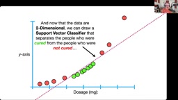
The core idea of SVM is: map low-dimensional data to a high-dimensional space through some transformation, and find a linear classifier in that high-dimensional space. For example, by adding a column of "dosage squared" as the y-axis to the dosage data, the one-dimensional data becomes two-dimensional, and the originally nonlinearly separable data can be separated by a straight line in two-dimensional space.
This transformation is not chosen arbitrarily; SVM systematically performs the mapping using kernel functions. Commonly used ones include the polynomial kernel (with parameter d controlling the polynomial degree) and the radial basis function kernel (RBF kernel, corresponding to an infinite-dimensional space).

The key is the kernel trick: the kernel function only computes the relationships between points in high-dimensional space without actually performing the transformation. This allows computations to be done on low-dimensional data while being equivalent to operations in high-dimensional or even infinite-dimensional space, greatly improving efficiency.
The choice of kernel function directly affects SVM performance. Commonly used kernels include the linear kernel, polynomial kernel, radial basis function (RBF) kernel, and Sigmoid kernel. The linear kernel is suitable for linearly separable or approximately linearly separable data, and is simple to compute with strong interpretability; the polynomial kernel controls the dimensionality of the mapping through parameter d and can capture interaction relationships between features, but numerical stability may deteriorate when d is large; the RBF kernel maps samples to an infinite-dimensional space and has strong nonlinear fitting capability, making it the default choice in many scenarios, but its parameter gamma requires careful tuning. In addition, kernel functions must satisfy Mercer's condition, i.e., the corresponding kernel matrix is positive semi-definite, which guarantees that the optimization problem has a global optimal solution. In practice, cross-validation is typically used to compare the performance of different kernel functions and parameters, combined with data size and feature dimensionality for selection.
Python Hands-On: Polynomial-Kernel SVM
Below we demonstrate SVM using scikit-learn on the diabetes dataset. The data contains two features, blood glucose and blood pressure, with the target variable being whether diabetes is present. For ease of visualization, only the blood glucose feature is used.
First, load the data and split it into training/test sets, then perform standardization. Standardization uses the mean and standard deviation of the training set to avoid data leakage.
from sklearn.preprocessing import StandardScaler
from sklearn.svm import SVC
from sklearn.metrics import confusion_matrix, accuracy_score
from sklearn.model_selection import train_test_split

X_train, X_test, y_train, y_test = train_test_split(X, y, test_size=0.2)
scaler = StandardScaler()
X_train_scaled = scaler.fit_transform(X_train)
X_test_scaled = scaler.transform(X_test)
Use a polynomial kernel with degree=2 and coef0=0.5, and fit the training data:
svm_poly = SVC(kernel='poly', degree=2, coef0=0.5)
svm_poly.fit(X_train_scaled, y_train)
y_pred = svm_poly.predict(X_test_scaled)

The evaluation shows an accuracy of about 68%. Considering the severe overlap in the data, this result is not too bad.
Since the kernel trick does not actually store the transformed coordinates, we manually construct a "blood glucose squared" column and then fit with a linear kernel to visualize the classification boundary. The linear-kernel model produces exactly the same confusion matrix and accuracy as the polynomial-kernel model, verifying the equivalence of the kernel trick.
After manually computing the slope and intercept, we can plot the parabolic data distribution and the linear classification boundary. The final model classifies all samples below the red line as 0 and those above as 1.
The complete code is available on GitHub, and learning alongside the StatQuest video is even more effective.
In SVM, standardization (StandardScaler) is a crucial preprocessing step because SVM's optimization objective depends on the Euclidean distances between sample points. If feature scales differ significantly, distance calculations will be dominated by features with large numerical ranges, causing the classification boundary to deviate. Standardization transforms each feature to a distribution with mean 0 and standard deviation 1, eliminating the influence of units. Note that you must call fit_transform only on the training set to compute the mean and standard deviation, and then use the same parameters to transform the test set; otherwise, information from the test set will leak into the training process, resulting in overly optimistic performance evaluation. In addition, parameters in the kernel function (such as degree and coef0 for the polynomial kernel, gamma for the RBF kernel) and the penalty coefficient C should be tuned using cross-validation grid search rather than relying on default values.
Key Takeaways
- The maximal margin classifier is sensitive to outliers; the soft margin improves generalization by allowing misclassifications
- The kernel trick computes high-dimensional relationships without actually increasing dimensionality, balancing efficiency and expressiveness
- The degree parameter of the polynomial kernel controls the mapping dimensionality and should be selected via cross-validation
- Standardization should be fit on the training set and transform applied to the test set to prevent data leakage
- Manual dimensionality increase + linear kernel can reproduce the SVM decision boundary for easier visualization and understanding
SVM has many terms, but the core logic remains consistent: when low-dimensional space cannot linearly separate the data, increase dimensionality to find a linear boundary. The kernel trick makes this process computationally feasible.
One-line Summary
SVM achieves nonlinear classification through maximal margin, soft margin, and the kernel trick, demonstrated with polynomial-kernel Python code.
Paragraph Summary
Based on StatQuest's explanation, this article systematically introduces the core concepts and practical applications of Support Vector Machines (SVM). Starting from the limitations of one-dimensional threshold classification, it introduces the maximal margin classifier and its sensitivity to outliers, then the soft margin and support vector classifier, achieving a bias-variance tradeoff by allowing misclassifications. For nonlinear problems, SVM uses kernel functions to map data to high-dimensional space, and the kernel trick avoids actual high-dimensional computations, improving efficiency. Finally, Python code demonstrates the complete workflow of a polynomial-kernel SVM on the diabetes dataset, including standardization, model training, evaluation, and decision boundary visualization, and verifies the equivalence of manual dimensionality increase and the kernel trick.
Related articles

Jon Krohn in Conversation: How LLMs Are Reshaping the Value of Data Scientists
Super Data Science host Jon Krohn talks with Josh Starmer and Luis Serrano about how LLMs erode twenty years of technical moats and shift value to context, business understanding, and agent orchestration.

Vergecast Ebook Library Tips: Multiple Virtual Library Cards and Kobo Integration
Vergecast shares ebook library tips: buy directly to support authors and indie bookstores, use multiple virtual library cards via Libby/Overdrive to expand library borrowing, and Kobo e-readers deeply integrate library resources with multi-card support.

GRPO Reinforcement Learning Explained: Group Relative Policy Optimization That Teaches LLMs to Reason
A deep dive into the GRPO reinforcement learning algorithm: how in-group relative advantages are computed, how clipping and the importance sampling ratio work in the loss, the role of KL divergence constraints, and GRPO's training-cost advantage over PPO—with round-by-round mathematical derivations.