KV Cache Saves 20x on Costs: The Underlying Principles and Practical Tips for LLM Inference Optimization

Same prompt, same model — the first call costs $1, the second costs just 5 cents — a full 20x cheaper. This isn't a bug; it's one of the most important cost optimization techniques in modern AI inference. What's even more interesting is that the underlying idea predates the Transformer itself, tracing back to a classic computer science concept from 1968.

Based on Adam Rosler's in-depth explanation, this article takes you from the fundamentals of how Transformers work to a thorough understanding of why KV Cache (Key-Value Cache) can dramatically shrink your API bill.

From Parallel Training to Sequential Inference: The Transformer's Inherent Bottleneck

Before 2017, language models could only process one word at a time, making training painfully slow. Google's team published the "Attention is All You Need" paper and completely rewrote the rules — every word could simultaneously attend to all other words in parallel, achieving a quantum leap in training speed.

The Transformer architecture proposed in this paper completely replaced the previously dominant RNN (Recurrent Neural Network) and LSTM (Long Short-Term Memory) approaches. RNN's fatal flaw was its sequential processing nature — computing the 100th word required waiting for all 99 preceding words to finish processing, making it impossible to fully leverage GPU parallel computing capabilities. Through the Self-Attention mechanism, Transformers allow every position in a sequence to simultaneously attend to all other positions, compressing training time from weeks to days. This architecture laid the technical foundation for all mainstream large language models that followed, including GPT, BERT, Claude, and others.

But here's the critical issue: inference (the process where the model generates a response for you) is still performed sequentially, step by step. Each new word depends on previously generated words, so during inference, the Transformer loses the advantage it was designed for — parallel computation.

To understand why inference is so expensive, we first need to grasp three fundamental concepts.

Three Core Concepts: Tokens, Embeddings, and Dot Products

Tokens — The Smallest Unit of Computation

When you send a prompt, the model first splits the text into tokens — sometimes whole words, sometimes fragments. This is the starting point for all computation.

Embeddings — Turning Words into Numbers

The model converts each token into a list of approximately 4,000 numbers, called its embedding vector. These numbers live in a large lookup table within the model file, with one entry per word, and these values are learned during pre-training. Inside the model, the word "CAT" isn't text — it's a list of 4,000 numbers.

The idea of embedding vectors dates back to Word2Vec, proposed by Mikolov et al. in 2013, with the core assumption that "a word's meaning is determined by the words around it" (the distributional hypothesis). Modern large models typically use embedding dimensions between 4,096 and 12,288 — GPT-4-class models may use 12,288 dimensions, while smaller models like LLaMA-7B use 4,096. Higher dimensions allow the model to capture more subtle semantic nuances, but computational and storage costs increase accordingly. Notably, these embeddings aren't static: unlike Word2Vec, embeddings in Transformers become context-dependent representations after passing through multiple attention layers, meaning the same word will have different final representations in different contexts.

Dot Product — Measuring Semantic Relevance

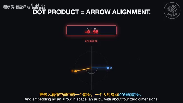
Think of an embedding as an arrow in space — about 4,000 dimensions, but let's compress it to 2D for visualization. The dot product of two arrows yields a single number: arrows pointing in the same direction produce a large positive value, perpendicular arrows yield 0, and opposite arrows produce a negative number.

Here's the elegant part: pre-training is essentially the model continuously adjusting embedding vectors until semantically related concepts point in similar directions. "CAT" and "KITTEN" point the same way; "CAT" and "YACHT" don't. Determining how related two words are becomes a matter of checking how well their arrows align. This idea isn't new — search engines have been using vector similarity since the 1970s.

The Attention Mechanism: Keys, Values, and Expensive Matrix Multiplications

For each token, the model computes two new vectors from its embedding, giving each token two roles:

• Key: What it advertises — "If you're looking for me, look here"
• Value: What it actually contributes — "If you pick me, take this"

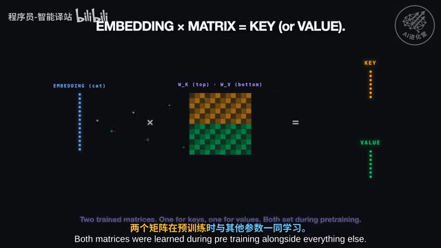
How are keys and values computed? By multiplying the embedding with a weight matrix. The model has two such matrices for Attention — one for generating keys, another for generating values — both learned during pre-training alongside other parameters.

The Query-Key-Value triplet in Attention borrows from information retrieval systems. A library analogy helps: the Query is the question in your mind when you walk into a library, the Key is the title and summary on each book's cover, and the Value is the actual content inside the book. You match your question against each book's title (dot product), find the most relevant books (high attention scores), and then primarily read those books' content (weighted sum).

In actual Transformers, there's another important detail: Multi-Head Attention. The model doesn't perform this query just once — it does it 32 to 128 times simultaneously (depending on model size), with each "head" focusing on different types of relationships. Some heads might focus on grammatical structure, others on semantic similarity, and others on positional relationships. This further amplifies computational load and makes KV cache optimization even more impactful.

To predict the next word, the model generates a Query, computes dot products with every previous Key to get attention scores, weights each Value vector by its score, then sums these weighted values — this sum becomes the input for predicting the next word.

But the hidden cost is that matrix multiplication operations are extremely expensive. Multiplying a 4,000-dimensional embedding by a 4,000×4,000 matrix means 16 million multiplications. The model consists of 40 stacked layers, each with its own Attention — across all 40 layers, setting up Attention for a single token requires approximately 2 billion operations.

KV Cache: Optimizing Modern AI Inference with a 1968 Memoization Idea

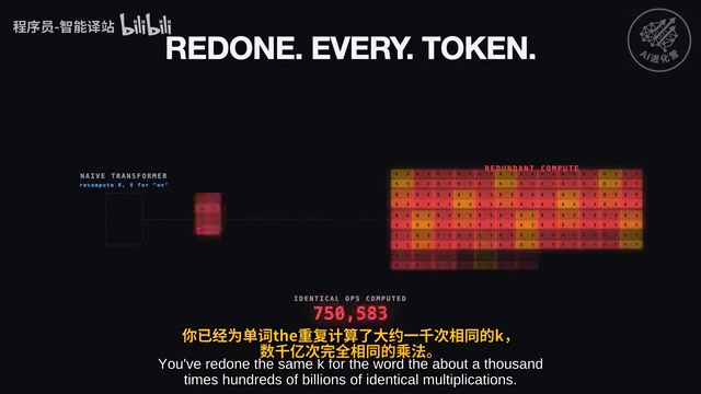
Here's the problem: a naive Transformer recomputes all previous tokens' keys and values when generating each new token. The same input prefix goes through the same matrices, producing exactly the same output. By the 1,000th token, you've redundantly computed the same key for the same word roughly 1,000 times — trillions of identical multiplications completely wasted.

Computer scientists noticed this waste as early as 1968. Donald Michie called it Memoization — save the answer, don't recompute.

The core principle of memoization is: if a function is pure (same input always produces same output), then after the first computation, store the result and return it directly from the lookup table for subsequent identical inputs. This seemingly simple idea is ubiquitous in computer science — from compiler optimizations and database query caches to CDN caching in web applications, they're all fundamentally the same principle. KV cache applies this classic idea to deep learning inference because the key-value computation in Attention happens to satisfy the pure function condition: the same embedding through the same weight matrix necessarily produces the same keys and values.

Applying memoization to the Attention mechanism gives us the Key-Value Cache (KV Cache). It's a set of saved key and value vectors from previously processed tokens, stored in GPU memory. After each token is processed, its keys and values are saved to the cache; the next token only needs to compute one new set of key-values, then runs Attention over the entire cache.

Why Cache Keys and Values Instead of Just Embeddings?

Because the embedding lookup itself is cheap — the expensive part is the matrix multiplication that transforms embeddings into K and V. What's costly is computing the intermediate results, not the input itself. Without KV cache, the generation process would consume roughly 1,000x more compute.

The Memory Cost of KV Cache

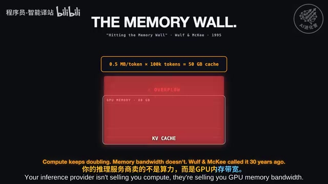
The cache itself has a cost: it lives in GPU memory and grows by one entry for every generated token. For a typical 70-billion parameter model, each token occupies about half a megabyte. Generate 100,000 tokens and you're carrying 50GB of cache — and each concurrent user has their own independent cache.

Computer architects warned about this problem back in 1995: compute power keeps doubling, but memory bandwidth hasn't kept pace. In their paper "Hitting the Memory Wall: Implications of the Obvious," Wm. A. Wulf and Sally A. McKee pointed out that processor speed improves about 60% per year while memory bandwidth improves only about 10% per year — a gap that causes compute capability to be severely bottlenecked by memory access speed. Nearly 30 years later, this problem has become particularly acute in AI inference. Take the NVIDIA H100 GPU as an example: it has approximately 80GB of HBM3 memory and about 3.35TB/s of memory bandwidth. When a 70-billion parameter model performs inference, generating each token requires reading model weights and KV cache data from memory. The bottleneck is often not the GPU's floating-point capability (~2000 TFLOPS) but how fast data can be moved from memory to compute units. Your inference provider isn't selling compute — they're selling GPU memory bandwidth.

Prompt Caching: From $1 to 5 Cents in Practice

Anthropic pioneered making KV cache reusable across API calls, calling it Prompt Caching. When you send a prefix identical to a recent request, the provider keeps your KV cache in GPU memory — subsequent requests only need to run Attention, with no extra matrix multiplication overhead and no repeated setup costs.

Anthropic launched this feature in 2024, followed by OpenAI, Google, and other major API providers. The specific pricing strategies reflect the underlying cost structure: taking Anthropic's Claude as an example, cache writes (building the cache for the first time) are typically priced 25% higher than standard input prices due to additional memory allocation and management overhead; cache hits (subsequent reuse) are priced as low as 10% of the standard price because the most expensive matrix multiplications are eliminated. Caches typically have a TTL (Time to Live), generally 5-15 minutes, after which they're cleared to free up precious GPU memory if no new requests hit them. This means prompt caching is best suited for high-frequency call scenarios like chatbots, agent loops, and batch processing tasks.

The first call pays for building the cache; the second call merely rents it. That's why the second call costs just $0.05 instead of $1.

The Golden Rule of Prompt Ordering

Understanding how KV cache works reveals a critically important practical tip: the order of content in your prompt matters enormously.

The correct approach is:

1. Put stable content first: system prompts, tool definitions, retrieved reference documents
2. Put variable content last: the user's actual question goes at the end

Why? Because keys and values at later positions depend on the model's processing of every earlier position through every layer. Changing anything in the prefix invalidates all cache entries from that point forward. If you move the user query to the front, your carefully built cache becomes worthless.

As long as the prefix remains unchanged, the cache can be reused for free with every request. Identical tokens, different order, vastly different cost implications.

Summary: Understanding the Truth Behind Your LLM API Bill

The cost structure of modern AI can be summarized in three statements:

• Long contexts are expensive — not because the model thinks harder, but because the KV cache is larger and occupies more GPU memory
• Repeated calls are cheap — because prompt caching avoids expensive redundant matrix multiplications
• Inference costs in agent loops can be reduced by 10x or more — provided you correctly organize your prompt order

Next time you design prompt templates for an AI application, remember this principle: put what doesn't change first, put what varies last. This simple adjustment might be the key to turning your API bill from astronomical to negligible.